What is Event Time in Stream Processing?
Stateful computation in Stream Processing
In stream processing, many use cases require computations that depend on time and state. For example, a VoD platform may want to display the most frequently watched movies within the last hour, while a financial service might need to count transactions in a given period to trigger fraud detection rules. Such scenarios are typically solved using time window aggregations or similar techniques.
These techniques rely on a clear notion of time – whether to assign an event to a window or to decide when a state can be safely discarded after a configured time-to-live (TTL) interval.
System Time vs Event Time
A straightforward approach is to use system time: the clock of the machine that processes the events. At first glance, this seems fine, but in practice, it often leads to unexpected results.
Imagine a device that loses its internet connection and only sends its data after it reconnects. The processing system will assign the delayed event to the current system time, not the time when the event actually happened. As a result, the event may end up in the wrong time window.
Another common situation is backfilling: replaying historical data to feed new logic. If system time is used, all replayed events would be treated as if they occurred “now,” making the results meaningless.
This is where event time comes in. Event time is the time when an event was originally emitted. Using event time ensures that computations accurately reflect reality, regardless of when the system received an event.
To address this, a stream processing solution should enable users to define the event time, and then all downstream components should utilise this time in their computational logic.
Event Time in Nussknacker
Like Apache Flink, the engine that powers it, Nussknacker is built with event time semantics at its core. This means:
- Sources in Nussknacker allow you to define the event time for incoming data.
- All stateful components in Nussknacker use event time consistently in their logic.
This ensures that computations are robust to delays, out-of-order arrivals, and reprocessing scenarios.
In the following sections, we’ll look at a concrete example of how vent time works in Nussknacker and how it helps to build reliable streaming scenarios.
The example: Tumbling window aggregation
Imagine we want to count incoming HTTP requests in 1-minute time windows for each user. During this aggregation, we want to consider the time of event creation rather than the time when events are ingested into Nussknacker. This could be important, for example, if our client device is a mobile device that can temporarily lose its internet connection. The picture below illustrates this. In this scenario, we added a timestamp field to show when the message occurred.

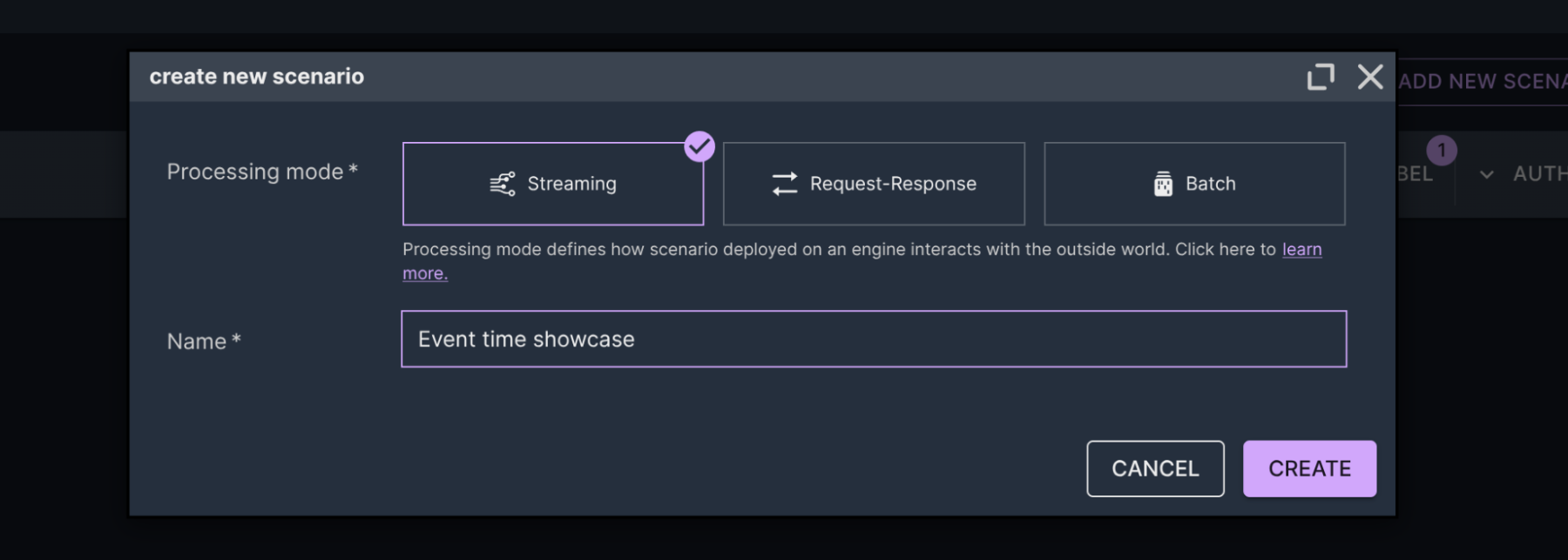
To realise this approach, we have to create a scenario.
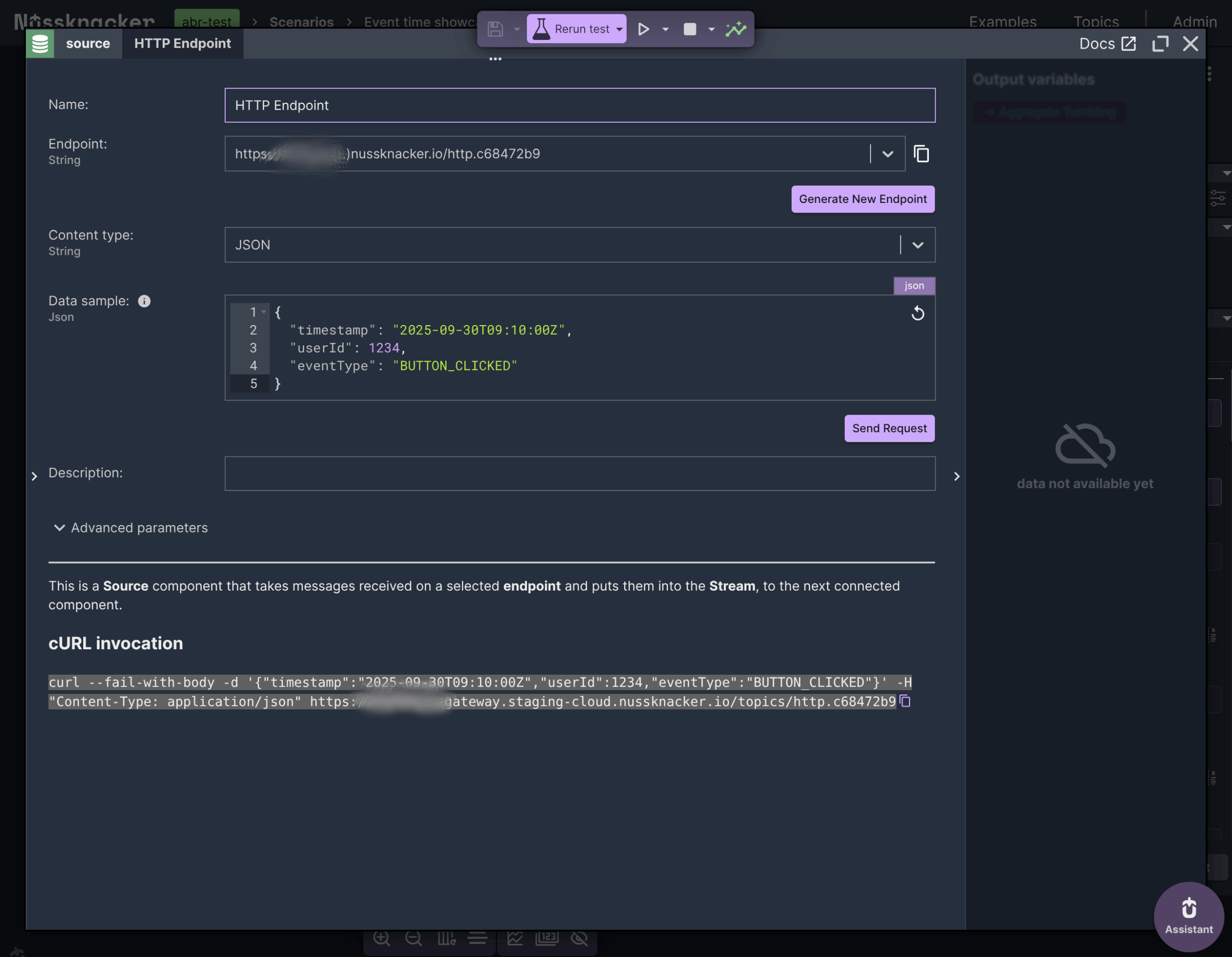
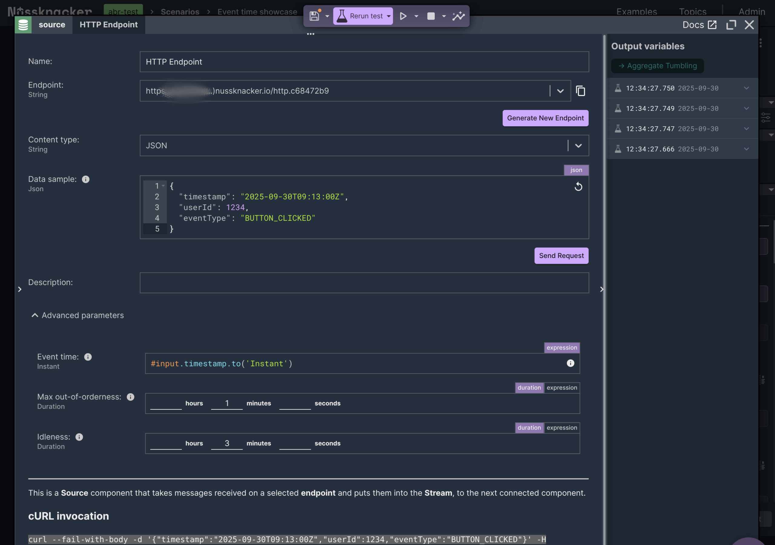
Then, we have to configure a source. In order to communicate with a scenario via HTTP in streaming mode, we use the HTTP Endpoint source. In the ‘Data sample’ parameter, we entered an example message to help Nussknacker determine the type of input variable and enable code completion.
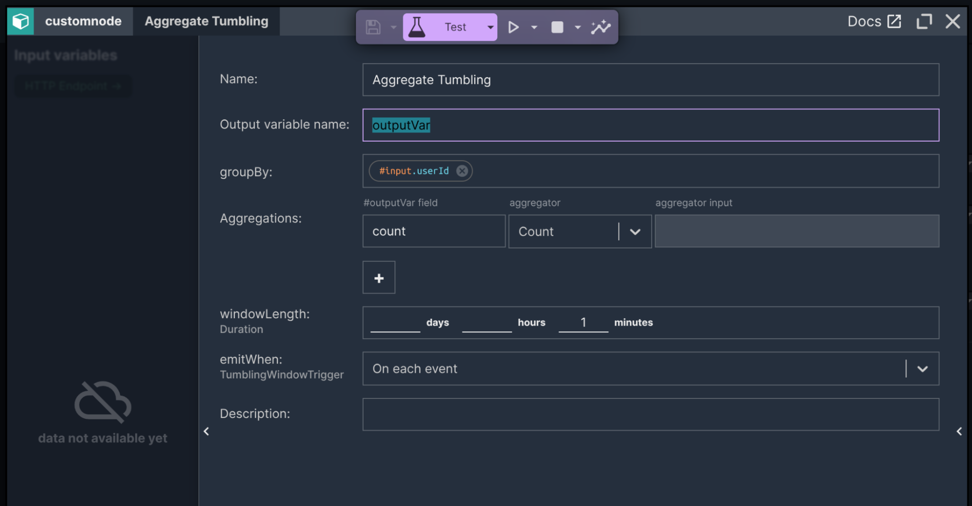
Next, we need to add an aggregation step.
Finally, we can deploy the scenario and test it live by either pressing the <Send Request> button available in the source node or invoking the cURL command available in the description below the source parameters.
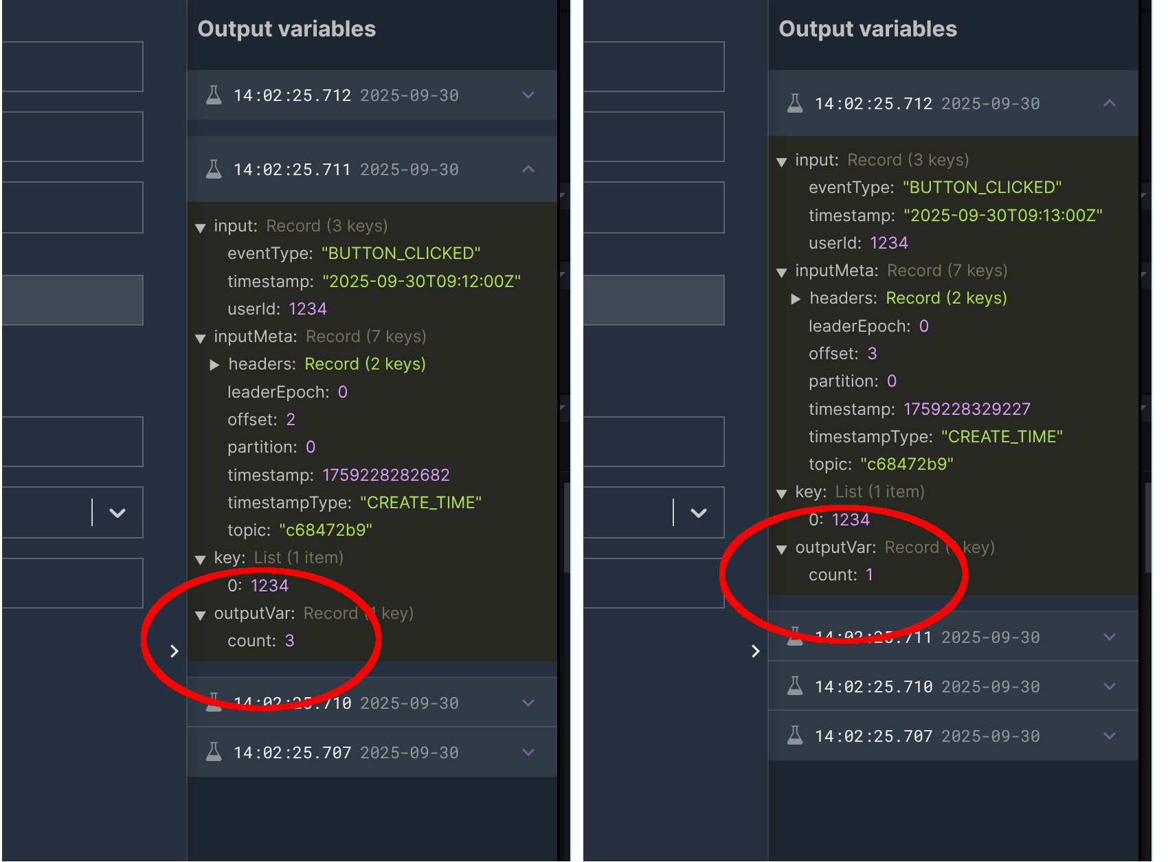
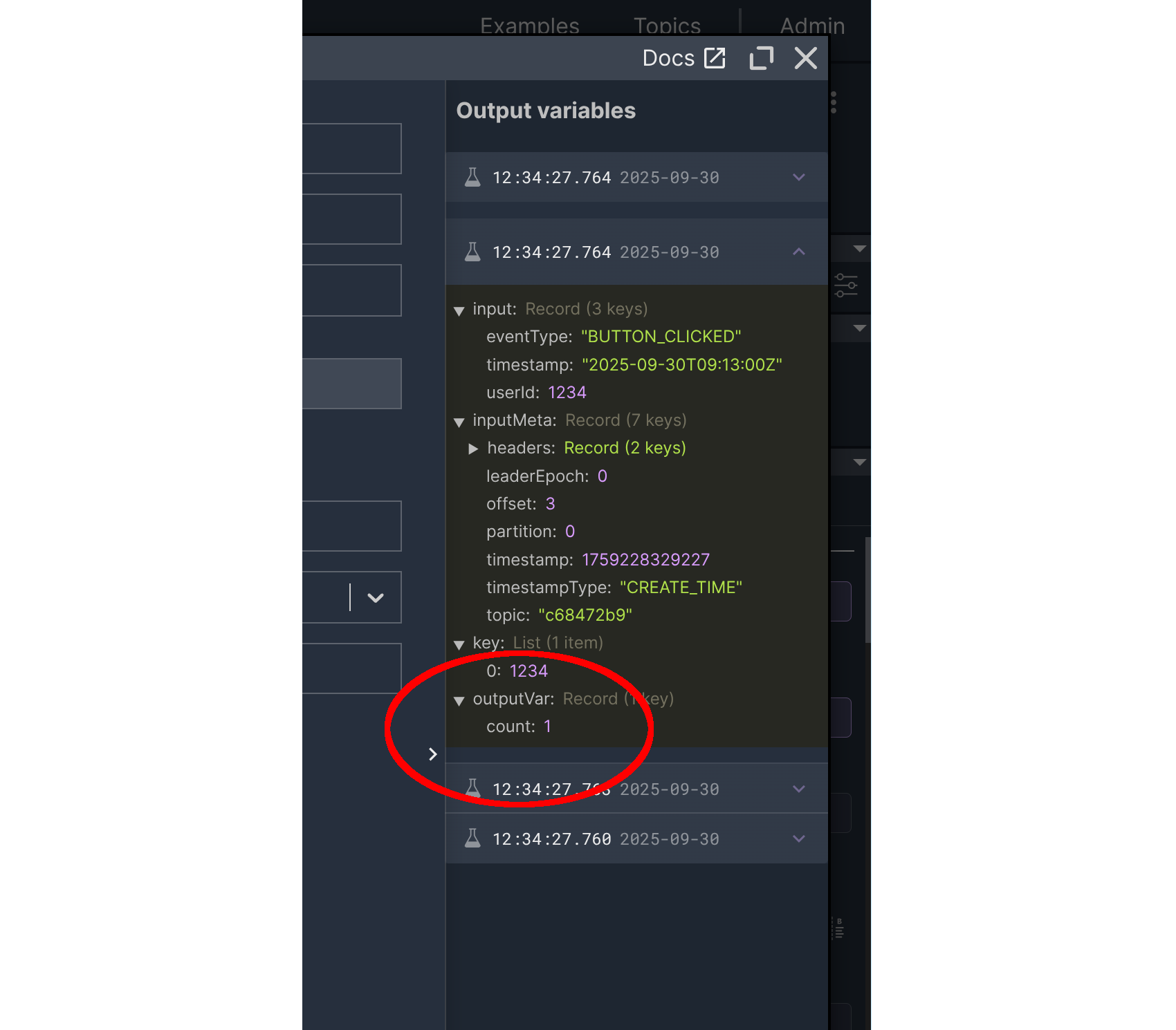
To verify the result of the aggregation, we can check the ‘Output variables’ panel on the right side of the Aggregate node. We sent three messages one by one, and then, after a short while, we sent a fourth message. The outputVar value shows 3 for the third message and 1 for the fourth. The first three messages were assigned to one tumbling window and the fourth to another.
In the scenario, we didn’t point to the timestamp field available in the message. Also, the timestamp value was the same for all four messages. So how did Nussknacker know the time of events? Was it the Wall-clock time? Let’s verify this using the <Test> button.
Replaying messages
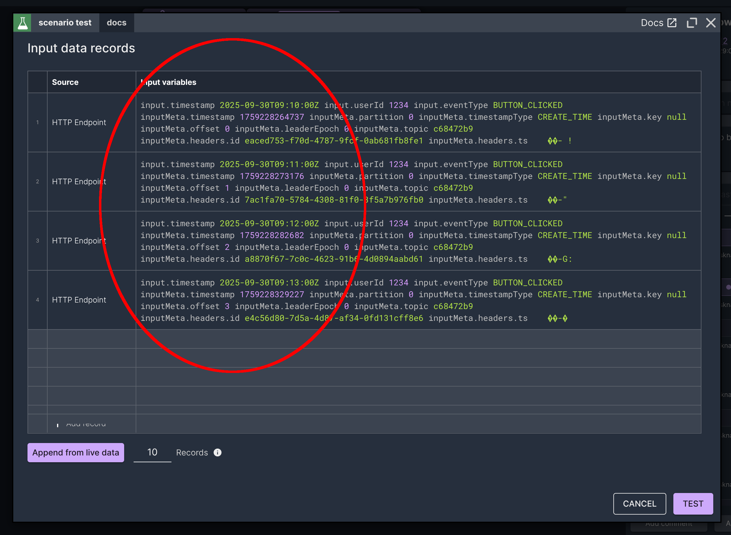
After clicking the <Test> button, we can see a table of input records that will be used during testing. Initially, the table is empty. We click the <Append from live data> button to fill it with live data.
We then click the <TEST> button to verify the results. We can see that the results in ‘Output variables’ are the same as they were when we sent real messages directly to the scenario. You might ask how this is possible. Taking a closer look at the data reveals that inputMeta.timestamp field contains a long number. For the first message, this value is 1759228264737. This value is in Epoch format, representing the number of milliseconds since 1 January 1970 and it can be displayed as 2025-09-30T10:31:04.737Z in ISO 8601 format. It contains the ingestion time – the time when an event was received by the Nussknacker Cloud platform.
When we come back to the Source node and click <Advanced parameters> button, we can see that 3 additional parameters, not visible at the beginning, are available.
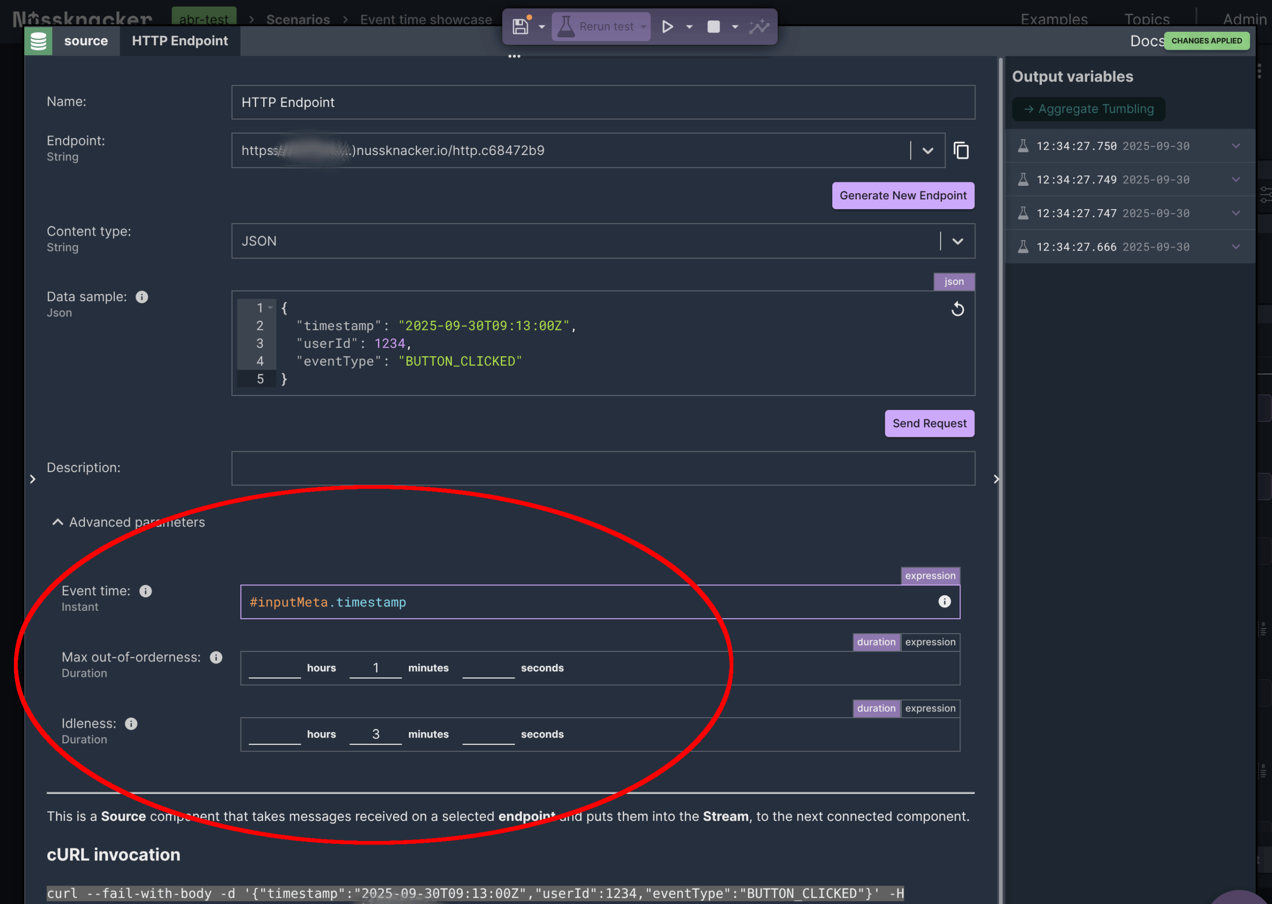
In the 'Event time' parameter, we can find the expression that determines event time. It uses the ingestion time mentioned above. However, we don’t want to use the ingestion time to emulate the situation described in the example. Instead, we have to switch to the timestamp field available in the message.
Using the correct Event Time
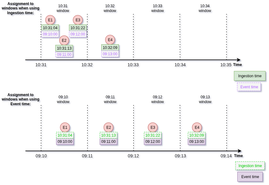
The illustration below shows two timelines: in the first timeline, you can see messages assigned to time windows based on the ingestion time. This is what we observed in the results so far. We have to switch to event time to observe the assignment visible in the second timeline.
To achieve this, we need to change the expression to #input.timestamp. The #input variable contains the payload that is sent in the HTTP body. The timestamp field contains the time filled during event emitting.
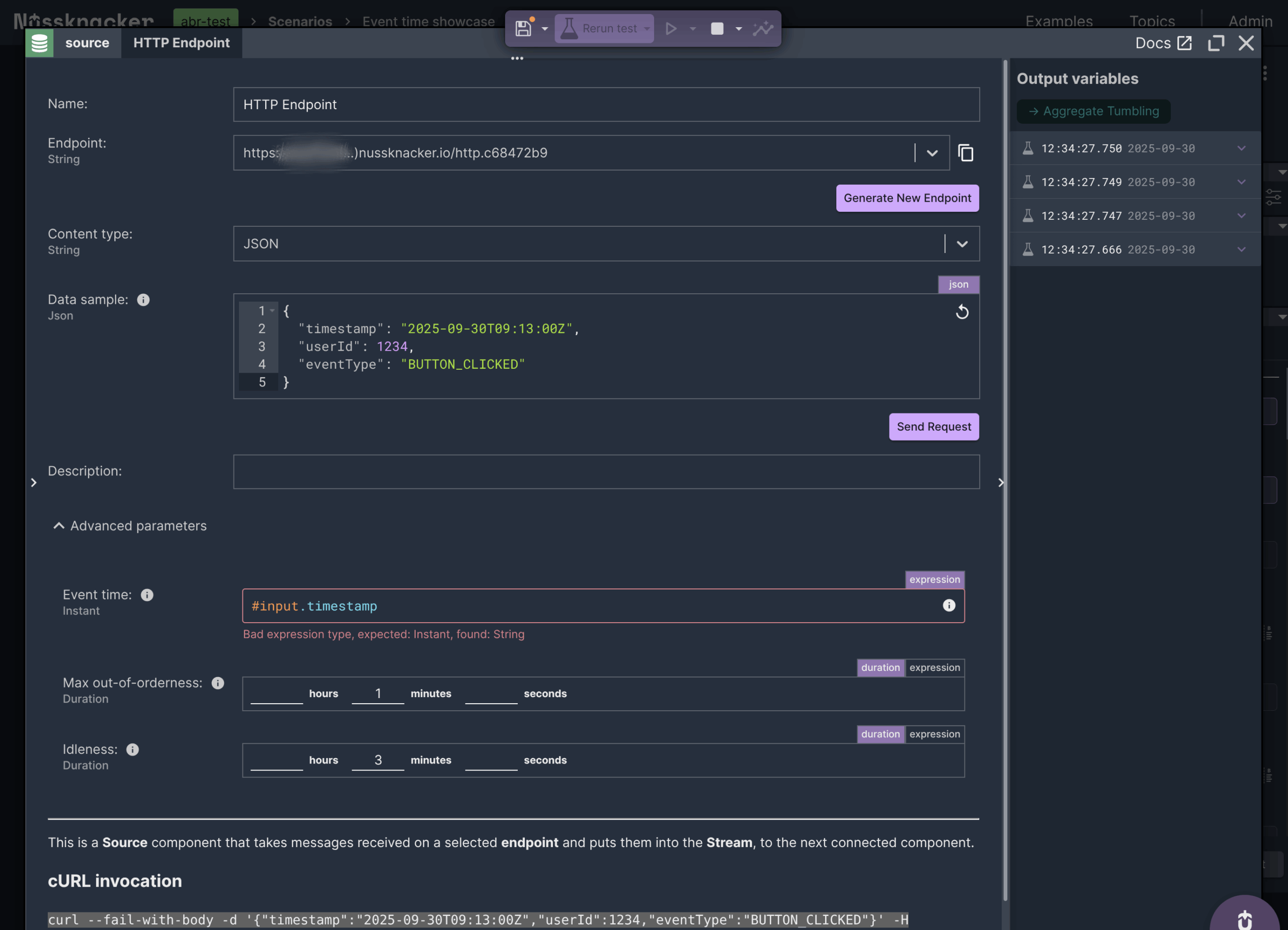
The Nussknacker’s Designer informs us that the type used in the expression is not an Instant. We need to tell it that it is not a bug – the timestamp field contains a timestamp in the correct, ISO 8601 format.
Now let’s <Rerun test> again and see what happens. We can see that now, for every message, the count shows 1 – the same situation as we showed on timeline 2.
Summary
Let’s sum up. Nussknacker components use event time during time window aggregations. This means that the result of the computation is the same whether a message is sent or replayed.
By default, this time is set up to ingestion time, which is suitable in many situations. For more advanced uses, you must send additional information about the timestamp
of the message and set the advanced parameter 'Event time' to this value.
Finally, there are two additional parameters worth knowing about: 'Max out-of-orderness' and 'Idleness'. They control how Nussknacker handles delayed or sparse events using the Watermarks mechanism – a fascinating topic that deserves its own deep dive, which we’ll explore in a future post.